Recently I’ve been working on a toy ray tracer to learn a bit about how 3D renderers work. I also took the opportunity to learn a little bit of math and a whole ton about computer graphics in general. This post isn’t a tutorial on how to build a ray tracer because there’s a ton of resources online already; it is mostly the journey I went through when writing Buzz, my toy ray tracer.

For the impatient, the source code of the whole project lives on github.

How it all started

More than a month ago I was watching Toy Story which is a thing I always love to do from time to time. That time I was particularly attracted by a scene where Buzz LightYear uses its laser to shoot rays everywhere to locate the enemies. That scene reminded me of how ray tracers work and so I decided to build one.

I don’t know very much about 3D and sure enough ray tracing was no exception, so the first thing I had to do was to gather some resources and read some documentation. To my surprise, I found out that a lot of ink has been spilled over this topic! After a bit of searching, I decided to follow Writing a Ray Tracer in a Weekend because it seemed a good compromise between theory and practice. I don’t regret this choice, but probably it was a bit too light on theory.

Ray Tracing 101

A ray tracer is a type of 3D renderer whose only purpose is to transform the description of a 3D scene into an image in the most accurate way possible. In order to do that it shoots a bunch of light rays into the scene and then it simulates how such rays reflect and refract to find out the color of every pixel in the final image.

If this sounds expensive to you, you’re right! It’s really way more expensive than rasterisation for example, but on the other hand the rendered image is way closer to reality especially when looking at shadows.

The core idea of the algorithm can be summarized by the following code snippet.

for (x, y) in output_image:
    for _ in 0..nsamples:
        color = shoot_ray(ray_going_through(camera, (x, y)))
        output_image.blend_pixel(x, y, color)

Quite neat, isn’t it? Obviously I’ve omitted where all the magic happens (that is in shoot_ray) but I think that is a good overview of how ray tracing works. It basically goes through each pixel of the final image, shoots slightly different rays into the scene and eventually blends all the potentially different colors for the same pixel.

The difficult part of ray tracing is in writing an efficient shoot_ray function. Conceptually, all it does is to find the closest intersection (if any) between the ray and the objects in the scene and then according to which object it hit and its material it calculates the color of the pixel.

Materials

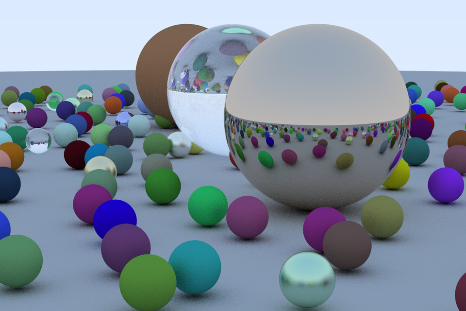
Coming up with a faithful representation of materials is hard and it turns out that this is very much a research area to this day. In fact there are a lot of ways to model materials with varying degrees of complexity and realism. I choose to implement only the lambertian(aka diffuse), metal and dielectric(aka glass) materials because they seemed the easiest to implement.

Among the three, the lambertian material was the easiest to implement because it turns out that a relatively good model consists in simply bouncing the incoming ray approximately along the normal of the intersected object. This ends up in simulating a perfectly diffuse material.

def lambertian_bounce(ray, obj):
    (intersection_point, normal) = obj.intersect(ray)
    return Ray(intersection_point, normal + randUnitVector())

Metal materials were a bit harder to implement because they do not simply make the incoming ray bounce in a random direction but instead such ray is reflected and then slightly perturbed. Intuitively this makes sense because pure metals simply reflect light rays.

def diffuse_bounce(ray, obj):
    (intersection_point, normal) = obj.intersect(ray)
    return Ray(intersection_point, reflect(ray.direction, normal) + randUnitVector())

Dielectric materials were the hardest to understand and to code. These materials look like glass and do not simply reflect incoming rays but instead they let some amount of rays go through the object (refraction) and others are reflected. The ratio between reflected and refracted rays are ruled by the Fresnel factor which I decided to simulate by using Schlick’s approximation equations. Practically this means that each time a ray hits a dielectric material Buzz randomly generates a probability and according to whether it’s greater or smaller than the Fresnel factor for that particular material it reflects or refracts the incoming ray. Quite mouthful I know, but hopefully the following code snippet will clarify things a bit.

def dielectric_bounce(ray, obj):
    intersection_point, normal = obj.intersect(ray)
    refracted_ray, cos = refract(ray, intersection_point, normal)

    if refracted_ray is None:
        return reflect(ray.direction, normal)

    reflect_prob = schlick(cos, refractive_index)

    if rand() < reflect_prob:
        return reflect(ray.direction, normal)

    return refracted

With just these three types of materials it’s possible to render quite interesting and pleasing scenes like the following even though the materials do not look very realistic because real materials are actually a mix of the diffuse, metal and dielectric components, but I’m ok with what I have for now.

Mesh

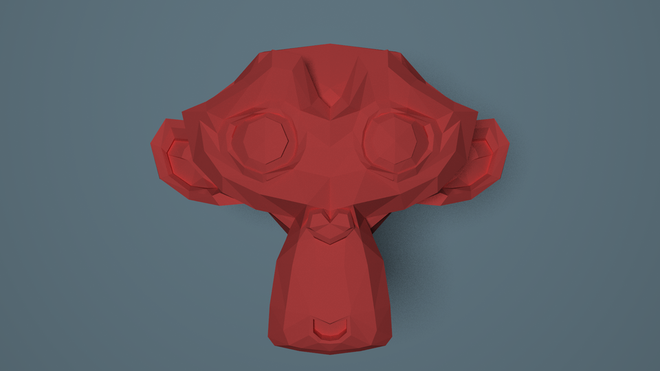
At this point I implemented pretty much everything that Ray tracing in a weekend covered, but I wasn’t satisfied yet. What I wanted to tackle next was to add support for rendering arbitrary meshes so that I would be able to render complex objects and not just boring geometric shapes.

It turned out to be quite simple because a mesh can be seen as just a collection of faces, triangles in my case, which share the same material. It’s not that different than inserting such faces directly in the scene as objects with the same material. In fact, that is basically what I do. I don’t know if it’s the most correct way to do this, but I think that it’s quite simple and gives good results.

Constructive Solid Geometry

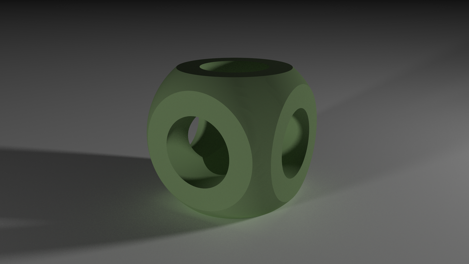
While studying ray tracers and in general learning more about 3D rendering I came across the concept of Constructive Solid Geometry or CSG. The core idea is to have simple primitive objects like spheres, cubes, etc… and then to use boolean operators (i.e. union, intersection and difference) to combine them together. Being a big fan of functional programming and composition in general, this concept really spoke to me and I decided that Buzz had to be able to render this kind of shapes.

The implementation was quite straightforward, I modelled the primitives using Signed Distance Functions or SDF. Signed distance functions are a way to look at objects as functions that return the distance from a point to the object’s surface. If the distance is negative then the point is inside the object, if it’s zero then it’s exactly on the surface and if it’s positive it’s outside the object. Here’s an example SDF for spheres

class Sphere:
    center: Vec3
    radius: float

    def dist(self, point):
        return (point - self.center).norm() - self.radius

Implementing the boolean operators on these primitives took me a bit of time, but I enjoyed the process nonetheless. The union between two SDF is simply the minimum distance between the two while the intersection is simply taking the maximum. Intuitively this means that the distance of a union object to a point is the distance of the closest object to that point and symmetrically for the intersection object. The difference operator is a bit more involved but it boils down to taking the intersection between the first object and everything but the second that is the intersection between the first object and the negation of the second. The negation can be done by simply changing the sign of a SDF.

def union(sdf1, sdf2, point):
    return min(sdf1.dist(point), sdf2.dist(point))

def intersection(sdf1, sdf2, point):
    return max(sdf1.dist(point), sdf2.dist(point))

def difference(sdf1, sdf2, point):
    return max(sdf1.dist(point), -sdf2.dist(point))

This is all pretty cool but unfortunately this isn’t enough to render CSG objects because usually ray tracers need to find the intersection point on the object to properly calculate the normal for shading, etc… However, CSG can only provide distances because that’s the whole point of representing models using SDF after all. Fear not though, there’s a technique known as ray marching that basically consists in moving along the incoming ray by its distance from the SDF object until such distance is 0 that is when the origin of the ray is the intersection point.

Using these simple operators it’s possible to describe quite complex objects like the following.

Conclusions

Ray tracers are pretty cool and are interesting to implement, but it’s not a walk in the park if you don’t know much about 3d math. The best part of this journey was that I could see the results of my code changes pretty much immediately because they almost always impacted the final images. I didn’t like debugging though, it’s super hard given that it’s not always obvious what’s causing weird effects in the final image.

There a lot of features missing in Buzz like textures and volume rendering, but I’m ok with what I have.

A feature that I’m considering adding is some very basic primitives to render animations given that I’m able to render images which can be seen as frames. However, since rendering a single good quality image takes a bit of time, I fear that making an animation of say 1 minute would require quite a bit of resources. It’d be pretty cool to produce short movies though.

Also, I might try to implement Physically based rendering at some point, but I’m done with ray tracing for the foreseeable future. The next thing is to build a rasterizer to explore the other face of 3D rendering. See you then.